Principal Component Analysis (PCA) is the most widely used multivariate technique in spectroscopy. It takes a dataset of spectra — each containing hundreds or thousands of wavenumber channels — and reduces it to a small number of principal components that capture the dominant patterns of variation. The result is a low-dimensional representation that reveals sample groupings, outliers, and the spectral features driving those differences.
This tutorial covers PCA from a practical spectroscopy perspective: what it tells you, how to interpret the output, and the preprocessing steps that make the difference between meaningful results and noise.
What PCA actually does
A spectrum with 1000 wavenumber points lives in 1000-dimensional space — one axis per channel. PCA finds a new coordinate system where the first axis (PC1) points in the direction of greatest variance in the dataset, the second axis (PC2) captures the most remaining variance orthogonal to PC1, and so on. Each successive component captures less variance than the one before it.
In spectroscopy, the first 3–10 principal components typically explain 95%+ of the total variance. The remaining hundreds of components represent noise, minor baseline variations, and other spectral artifacts. By projecting the data onto just the first few PCs, you collapse the dimensionality from thousands of channels to a handful of meaningful variables.
This is not just data compression. The PCA decomposition separates signal from noise and reveals structure that is invisible when looking at raw spectra stacked on a plot.
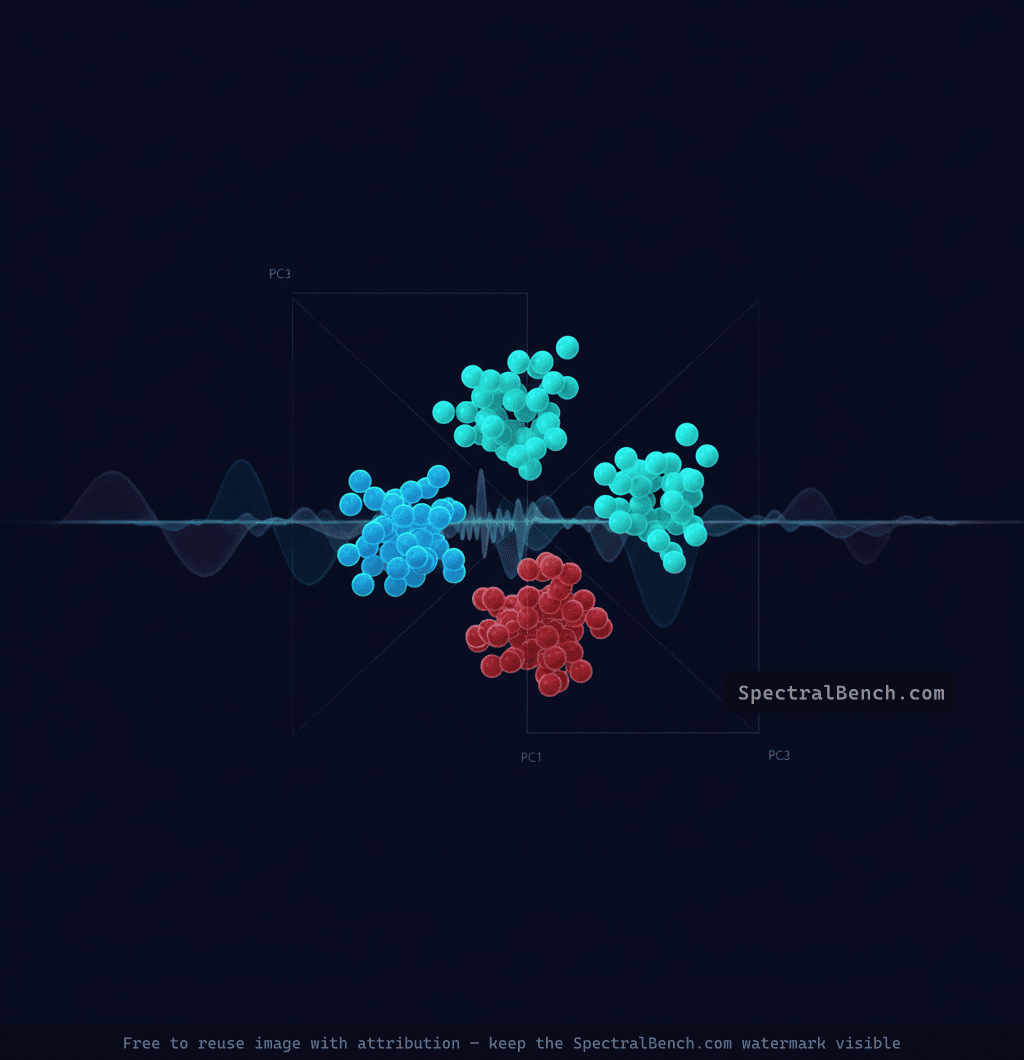
Scores: where samples sit
The scores are the coordinates of each sample in the new PC coordinate system. A scores plot (typically PC1 vs. PC2) shows each spectrum as a single point in a 2D scatter plot.
Interpreting scores plots
Clusters indicate groups of similar samples. If your dataset contains spectra from three different polymer types, you expect to see three distinct clusters in the scores plot. The tighter the cluster, the more internally consistent that group is.
Separation between clusters indicates spectral differences. Large separation means the groups have substantially different spectral features. Small separation means the differences are subtle relative to within-group variation.
Outliers — points far from any cluster — indicate unusual spectra. These could be measurement artifacts (poor contact in ATR, baseline drift), contaminated samples, or genuinely novel compositions. Always investigate outliers before removing them.
Gradients — continuous variation rather than discrete clusters — indicate a continuous property change. For example, spectra of polymer blends at different mixing ratios will show a smooth gradient between the pure-component clusters rather than discrete groupings.
PC selection matters. PC1 vs. PC2 shows the two directions of greatest variance, but these may not be the directions that separate your groups of interest. If PC1 captures baseline variation (common in poorly preprocessed data), the grouping information may only appear in PC2 vs. PC3 or higher components. Always explore multiple PC combinations.
Loadings: what drives the differences
The loadings describe what each principal component represents in terms of the original spectral variables. A loadings plot for PC1 shows the weight (positive or negative) assigned to each wavenumber channel — it tells you which spectral features contribute most to the variation captured by that component.
Interpreting loadings plots
Peaks in the loadings correspond to wavenumber positions where the spectra differ most. A positive loading at 1714 cm⁻¹ on PC1, for example, means that samples with high PC1 scores have stronger absorption at 1714 cm⁻¹ (the carbonyl region), and samples with low PC1 scores have weaker absorption there.
The sign is relative. A positive loading means "more absorption correlates with positive scores direction." The direction of the PC axis is arbitrary — PCA might flip the sign. What matters is the pattern: which peaks load together (same sign) and which load oppositely.
Noise in the loadings indicates that the corresponding PC is capturing noise rather than signal. If the loadings plot for PC5 looks like random noise with no identifiable spectral features, that component is not contributing meaningful chemical information.
Derivative-like loadings patterns (a peak with a positive lobe adjacent to a negative lobe) indicate that the corresponding PC is capturing peak shifts rather than intensity changes. This commonly occurs when samples have the same functional groups but in slightly different chemical environments.
Explained variance: how many PCs to keep
The explained variance ratio tells you what fraction of total spectral variance each component captures. Plot the cumulative explained variance against PC number to create a scree plot.
The practical rule
Keep enough components to explain 95–99% of the total variance. The scree plot typically shows a sharp drop after the first few components, followed by a long, flat tail of noise components. The "elbow" at the transition is your cutoff.
For a typical FTIR dataset:
- PC1 might explain 70–90% of variance (dominant spectral differences)
- PC2 captures 3–15% (secondary differences)
- PC3–PC5 capture 1–5% each (finer distinctions)
- PC6+ capture < 1% each (noise)
Including too many components overfits to noise. Including too few discards real spectral information. When in doubt, err on the side of fewer components and check whether the loadings of borderline PCs show recognizable spectral features.
Preprocessing: the step that matters most
The most common PCA mistake in spectroscopy is applying PCA to raw, unprocessed spectra. Baseline variations, intensity scaling differences, and scattering effects can dominate the first principal components, pushing the actual chemical information into higher PCs where it is harder to find and less reliably separated from noise.
Essential preprocessing steps
Mean centering (subtract the mean spectrum from every spectrum in the dataset) is mandatory. Without mean centering, PC1 simply represents the average spectrum rather than the primary direction of variation. Every PCA software tool should apply this by default.
Standard Normal Variate (SNV) normalization removes multiplicative scatter effects by centering each spectrum to zero mean and scaling to unit standard deviation. This is critical for solid-sample FTIR and diffuse reflectance measurements where particle size and packing density affect overall intensity without changing peak positions. Apply SNV before mean centering.
Savitzky-Golay derivatives (first or second derivative) remove baseline offsets and enhance spectral resolution. First derivatives remove constant baseline offsets; second derivatives remove linear baseline slopes and sharpen overlapping peaks. The tradeoff is increased noise — choose the polynomial order and window width carefully.
Spectral range selection — restrict the analysis to the informative region. Exclude noisy ranges (below 400 cm⁻¹ in FTIR), the CO₂ absorption region (2300–2400 cm⁻¹ if purge is inadequate), and any region dominated by a single overwhelming peak (like the diamond ATR absorption around 2000 cm⁻¹).
Preprocessing order
A robust preprocessing pipeline for FTIR spectral PCA:
- Spectral range selection
- Baseline correction (rubber band or polynomial)
- SNV normalization
- Optional: Savitzky-Golay smoothing or derivatives
- Mean centering (applied by the PCA algorithm)
The order matters. Normalizing before baseline correction can amplify artifacts. Taking derivatives before smoothing amplifies noise.
When PCA is the right tool
PCA excels at:
- Exploratory analysis — visualizing structure in a new dataset before applying supervised methods
- Quality control — detecting outlier batches that deviate from the normal production range
- Classification preprocessing — reducing dimensionality before feeding data into classifiers (SVM, random forest, neural networks)
- Identifying the source of variation — loadings reveal which functional groups or spectral features drive observed groupings
When PCA is not enough
PCA is unsupervised — it finds the directions of greatest variance regardless of whether those directions are relevant to your classification problem. If the variance between groups is small relative to within-group variance (e.g., subtle compositional differences against a noisy background), PCA may not separate the groups at all.
For supervised problems where you have labeled training data, consider:
- PLS-DA (Partial Least Squares Discriminant Analysis) — maximizes the covariance between spectra and class labels, rather than maximizing variance. Better separation when class differences are subtle
- LDA (Linear Discriminant Analysis) — maximizes the ratio of between-class to within-class variance. Requires more samples than variables, so often applied after PCA dimensionality reduction
PCA also assumes that the data structure is linear. For datasets with complex, non-linear relationships between spectra, t-SNE or UMAP may reveal groupings that PCA misses — though these non-linear methods sacrifice the interpretable loadings that make PCA so valuable.
Practical example
Consider a dataset of 100 FTIR spectra from five different plastic types collected during a recycling sorting study. Raw spectra show obvious differences (PE vs. PET) and subtle ones (HDPE vs. LDPE). After SNV normalization and mean centering:
- PC1 (78% variance) separates polymers with carbonyl groups (PET, nylon) from pure hydrocarbons (PE, PP, PS). The loadings peak at 1714 cm⁻¹ (C=O) and 1240 cm⁻¹ (C-O-C ester)
- PC2 (12% variance) separates aromatic polymers (PS, PET) from aliphatic ones (PE, PP, nylon). The loadings show aromatic C-H stretches (3026 cm⁻¹) and ring modes (1600, 698 cm⁻¹)
- PC3 (4% variance) separates HDPE from LDPE based on crystallinity differences in the CH₂ rocking region (730/720 cm⁻¹ doublet)
The first two PCs alone classify 4 of the 5 polymer types correctly. Adding PC3 resolves the PE subgroups. This is the power of PCA — reducing 1000 spectral channels to 3 interpretable variables that map directly to chemical differences.
Try running PCA on your own spectral datasets using SpectralBench's built-in PCA tool — load multiple spectra and visualize scores and explained variance instantly, with no software installation required.